
 Create Graphs and Charts in Excel 365
By Shannon Glennon
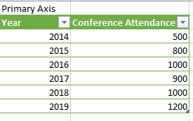
Format your dataset as a table, and select it.
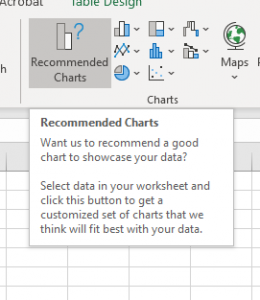
Click on the Insert Tab
First, check out the Recommended Charts for a customized set of charts that Microsoft detects will best suit your dataset.
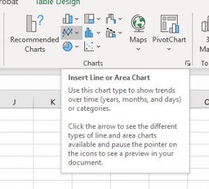
To create a custom chart instead, select Insert, and one of the options in the Charts group. For this example, I’m selecting a Line or Area Chart.
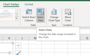
There are several ways to customize your chart to work with your dataset. Select the chart to open the Chart Design contextual tab. Click on Select data.
In the Select Data Source dialogue box, you’ll notice the bottom left are your different line charts. For this chart, I’m going to remote the year, because that simply results in a straight line as it advances throughout the years. To do this, select year, then click remove.
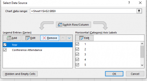
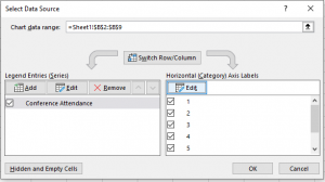
I do wish to map out the Conference attendance over time, so I’ll leave that as a Legend Entries (Series). Now you’ll notice on the right side of the Select Data Source dialogue box, the Horizonal Axis Labels list numbers from 1 to 6 currently. For this chart, I want this to be the year, so I’ll click Edit.
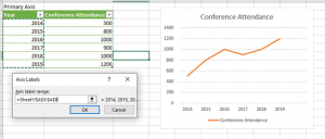
I would like the Axis label range to be the year, so I’ll highlight the years in my chart (notice the years already appear at the bottom of the chart), then click Ok.
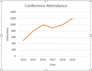
To add labels, on the Chart Designs contextual tab, click on Add Chart Element, Axis Titles.
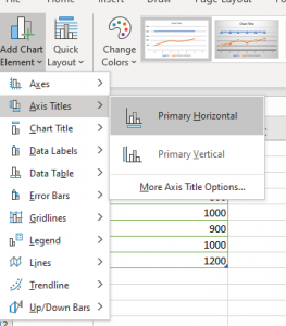
After adding labels to the chart, your chart will appear like this.
If you have questions or would like more in depth training for charts with a Secondary Axis, or other formatting options, please email icttraining@syr.edu.